More fun with simulation
Let's try to reproduce the data from the NFkB paper. To do this, we need to learn how to implement more complicated inputs, and how to simulate a model to steady state before applying an input.
Contents
Implicit input functions
Instead of just specifying the constant value for the input as a function of time, we can define any function that takes an input t and passes a column vector as an output.
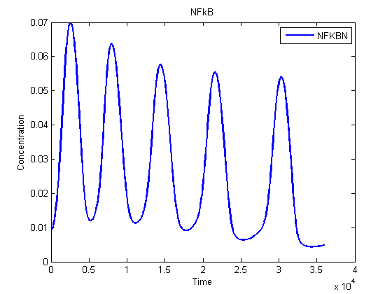
Let's see if the NFkB network acts like an excitable system. To do this, we make an input function u(t) that turns off at some time of interest. Then, we run constructExperiment with tF and u, and also let it know any times at which this time-varying input will change discontinuously.
tF = 3600*10;
tOff = 6000;

u = @(t) [1e-5*(t<tOff)
                      1
                      0
                      0];

expt = constructExperiment(tF, u, tOff);
simulate(m, expt);
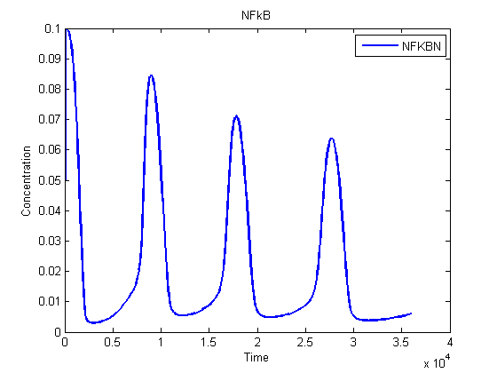
Simulating to steady state
This is just a simple application of the tools you've already gotten. Let's simulate with TNFa = 0 and then set m.ic, the model's initial conditions, to the value of the state variables at the final timepoint.
tSS = 3600*100; % 100 h should get us close to steady state
expt_ss = constructExperiment(tSS, [0;1;0;0]);
[t y x] = simulate(m, expt_ss);

m.ic = x(3600*100);

simulate(m, expt)