Demo Dose Response Command

This scripts demonstrates how to use the doseResponse command. This command is used to find the steady state concenetrations for a model given a particular input u. Mathematically this means solving for x that is consitent with the initial conditions such that:

We solve this equation using Newton's method which allows the method to find both stable and unstable fixed points.
Contents
Load the model
First we load the model using the loadModel command. In this case it is a model of a distributive MAPK phosphorylation dephosphophorylation loop.
model = loadModel('OneStepMAPK');
exp       = constructExperiment(10000, 0.01);
[t, y, x] = simulate(model, exp, struct('rel_tol', 1e-9, 'abs_tol', 1e-12));
Compute the dose response curve
We solve for the steady state concentration of the system over a range of kinase concentrations u. The output is the steady state concentration as well as the residulat of the steady state equation.
u               = logspace(-2, 2, 100);
[yss, xss, val] = doseResponse(model, u, x(t(end))');
Plot Results
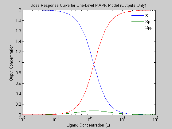
We plot the dose response curves for the System outputs, in this case the unphosphorylated substrate (S), the singly phosphorylated substrate (Sp) and the doubly phosphorlated substrate (Spp). The second plot shows the dose response curves of all of the model species.
figure;
semilogx(u, yss,  '-');
legend(model.yNames);
xlabel('Ligand Concentration (L)');
ylabel('Ouput Concentration');
title('Dose Response Curve for One-Level MAPK Model (Outputs Only)');