Demo Dose Response Command

This scripts demonstrates how to use the doseResponse command. This command is used to find the steady state concentrations for a model given a particular input u. Mathematically this means solving for x that is consistent with the initial conditions such that:

We solve this equation using Newton's method which allows the method to find both stable and unstable fixed points.

Contents

Load the model

First we load the model using the loadModel command. In this case it is the Huang & Ferrell model of the MAPK cascade.

model = loadModel('ThreeStepMAPK');

exp       = constructExperiment(10000, 0.01);
[t, y, x] = simulate(model, exp, struct('rel_tol', 1e-9, 'abs_tol', 1e-12));

Compute the dose response curve

We solve for the steady state concentration of the system over a range of kinase concentrations u. The output is the steady state concentration as well as the residual of the steady state equation.

u               = logspace(-2, 3, 100);
[yss, xss, val] = doseResponse(model, u, x(t(end))');

Plot Results

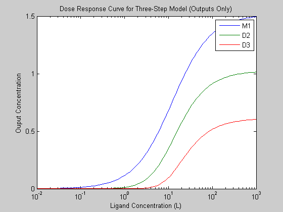
Again, we plot the dose response curves for the system outputs. In this case, the outputs are the active MAPKKK, MAPKK, and MAPK species.

figure;
semilogx(u, yss,  '-');
legend(model.yNames);
xlabel('Ligand Concentration (L)');
ylabel('Ouput Concentration');
title('Dose Response Curve for Three-Step Model (Outputs Only)');

Published with MATLAB® 7.2