Day 3, part 1: Loading and simulating the model again
In this section, we'll re-load and simulate the NFkB model adapted from [1]. Because we'll be interested in both sensitivities with respect to concentration and time today, we'll implement an 'events function' to compute the timing of nuclear NFkB pulse maxima.
Contents
Load the model
Once again, we'll be analyzing the NFkB model.
m = loadModel('NFkB');
Construct the experiment
We will parameterize the model with the same input we did yesterday.
u = @(t) [1e-3/(1+t/100)^2; 1; 0; 0];
As we did yesterday, let's set the final simulation time to 7 hours after TNFa stimulation.
tF = 3600*7;
Recall that yesterday we used an event that marked the NFkB peak time. We then used this event to construct an experiment that simulated the network for three pulses.
events = constructEventOutputPeak(m);
expt = constructExperiment(tF, u, [], events, 5);
Running and plotting the simulation
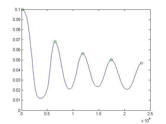
Next, we're going to simulate this input, and take a more detailed look at the output from a simulation.
simulation = simulate(m, expt);
plot(simulation.t, simulation.y(simulation.t), simulation.te, simulation.ye, 'o')
References
[1] Hoffmann A, Levchenko A, Scott M, Baltimore D. Science 298(5596):1241-1245 (2002).