Day 3, part 3: Other types of sensitivity analysis
In this section, we'll try two other types of sensitivity analysis. * Full forward sensitivity calculation * Sensitivities to the timing of a concentration's maximum or minimum
Contents
Computing *full* forward sensitivities
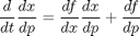
Sometimes you're not just interested in the value of a species or output at a particular timepoint, but instead want the continuous sensitivity as a function of time.
This problem can be solved by solving differentiating the model

with respect to parameters to obtain
We'll first modify the experiment to run for a shorter time, as we don't want you to have to wait forever for this line to run!
expt = constructExperiment(tF, u, [], events, 3); % <--- only run for 3 events, instead of 5
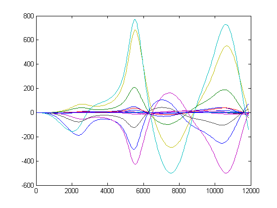
[dydp dxdp t] = sensitivity_state(m, expt);
plot(t, dydp(t))
Computing sensitivities with respect to timings
Again, we're going to use one of KroneckerBio's builtin objective functions. The math for computing the sensitivities of event timings is actually somewhat involved; see [2] for an introduction to these sorts of issues.
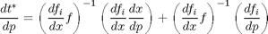
For the system


it can be shown that
This is what constitutes the guts of the constructObjectiveTiming functions.
expt = constructExperiment(tF, u, [], events, 5);   % <--- run for 5 events again
obj = constructObjectiveTimingOutputValue(m, 1, 2);
[O dOdp] = sensitivity(m, obj, expt);
rankSensitivities(m, dOdp, 10)
Param #		Name			Value			dGdp
-------		----			-----			----
  32		tp1  		   0.00015		 -1.6e+007
   6		tr3  		   0.00028		-1.22e+007
  40		k02  		   0.00012		 7.63e+006
   1		tr1  		  0.000408		  3.9e+006
  30		deg1 		  0.000113		-3.51e+006
  42		DNAprod		     0.001		 1.59e+006
  29		k01  		    8e-005		-8.51e+005
  31		deg4 		 2.25e-005		-6.59e+005
  22		r1   		   0.00407		-3.36e+005
  19		d4   		    0.0005		 3.27e+005
References
[2] Wilkins KA, Barton PI, Tidor B. PLoS Comp Biol 3(12):e242 (2007).